10X genomics scRNA-seq alignment

Python

Bioinformatics

scRNA-seq

Cellranger

Author

Taeyoon Kim

Published

February 21, 2024

Modified

June 30, 2025

1 들어가며

다음과 같은 몇가지 가정을 하고 시작하겠습니다.

가정1. 10x Genomics Single Cell Solution을 통해 얻은 서열 데이터를 사용 가정2. 리눅스(Ubuntu 22.04.3 LTS x86_64) OS를 사용하며 기본적인 shell 명령어를 앎 가정3. 패키지 매니저인 Anaconda에 대한 사용법을 알고 있음 터미널을 열고 원하는 폴더로 이동합니다. 저는 /home/fkt/Downloads에서 시작하도록 하겠습니다.

$pwd
/home/fkt/Downloads

터미널을 열고 원하는 폴더로 이동합니다. 저는 /home/fkt/Downloads에서 시작하도록 하겠습니다. 저는 아래와 같은 가정을 한 상태로 진행합니다.

1.1 가상환경 사용하기

정확하게는 velocyto를 사용하기 위해 가상환경을 만들어 사용합니다. 먼저 TutorialEnvironment.yml 파일을 다음 명령어로 다운받습니다.

wget https://cf.10xgenomics.com/supp/cell-exp/neutrophils/TutorialEnvironment.yml

다음 명령어로 가상환경을 만들어 줍니다.

conda env create --file TutorialEnvironment.yml

만들어진 가상환경을 활성화 시킵니다.

conda activate tutorial

다운로드 받은 yml파일은 삭제해줍니다.

rm TutorialEnvironment.yml

2 Cellranger 설치

자세한 것은 https://www.10xgenomics.com/support/software/cell-ranger

2.1 System Requirements

Hardware Cell Ranger pipelines run on Linux systems that meet these minimum requirements:

8-core Intel or AMD processor (16 cores recommended).
64GB RAM (128GB recommended).
1TB free disk space.
64-bit CentOS/RedHat 7.0 or Ubuntu 14.04 - See the 10x Genomics OS Support page for details.

2.1.1 Cell Ranger 7.2.0 (Sep 13, 2023)

Chromium Single Cell Software Suite Self-contained, relocatable tar file. Does not require centralized installation. Contains binaries pre-compiled for CentOS/RedHat 7.0 and Ubuntu 14.04. Runs on Linux systems that meets the minimum compute requirements.

다음 명령어를 통해 cell ranger를 다운로드 합니다.

wget -O cellranger-7.2.0.tar.gz "https://cf.10xgenomics.com/releases/cell-exp/cellranger-7.2.0.tar.gz?Expires=1695129121&Key-Pair-Id=APKAI7S6A5RYOXBWRPDA&Signature=ZipqR8Pg4YvVDQ3MvAVuuiPwEOC5c39~Wj0WTAxfoJW6xtrxqIFgIDySFSFnsWcwDpmAovJGrHXU24Y9Cptt88OJSPdEupyFRXoGKJvVzRtDJChmuMbSpVCy-2N-QnMKwxNtd8Yt8Mdp2Vcq4wxx1hVC0Yx54c7U9o~RFXIVsIp48thKR6JnKhJmCAC5U4dFLa86~NcB4s5Ic4HATrQP2KyWexyYZWgmBEw13mlKYtlVRUil0zseoq0-CZyGmE8oB0iDBSUBAyIqo~XMVjv~lkMz4cRcyCbQKBRDr~U36FM2KnE3rhv-Rlp4KD-uXCReRnBsY6N6t-HxpS2YDpN3mQ__"

그리고 나서 다음 명령어로 압축을 풀어줍니다.

tar -xvf cellranger-7.2.0.tar.gz

cellranger-7.2.0 폴더로 이동하기

cd cellranger-7.2.0

정상적으로 되었다면 아래와 같은 폴더 구조를 볼 수 있습니다.

.
├── bin
├── builtwith.json
├── cellranger -> bin/cellranger
├── external
├── lib
├── LICENSE
├── mro
├── probe_sets -> external/tenx_feature_references/targeted_panels
├── sourceme.bash
├── sourceme.csh
└── THIRD-PARTY-LICENSES.cellranger.txt

5 directories, 6 files

이제 ./cellranger명령어를 입력하면 아래와 같이 cell ranger 실행이 가능합니다.

./cellranger
cellranger cellranger-7.2.0

Process 10x Genomics Gene Expression, Feature Barcode, and Immune Profiling data

Usage: cellranger <COMMAND>

Commands:
  count           Count gene expression and/or feature barcode reads from a single sample and GEM well
  multi           Analyze multiplexed data or combined gene expression/immune profiling/feature barcode data
  multi-template  Output a multi config CSV template
  vdj             Assembles single-cell VDJ receptor sequences from 10x Immune Profiling libraries
  aggr            Aggregate data from multiple Cell Ranger runs
  reanalyze       Re-run secondary analysis (dimensionality reduction, clustering, etc)
  mkvdjref        Prepare a reference for use with CellRanger VDJ
  mkfastq         Run Illumina demultiplexer on sample sheets that contain 10x-specific sample index sets
  testrun         Execute the 'count' pipeline on a small test dataset
  mat2csv         Convert a gene count matrix to CSV format
  mkref           Prepare a reference for use with 10x analysis software. Requires a GTF and FASTA
  mkgtf           Filter a GTF file by attribute prior to creating a 10x reference
  upload          Upload analysis logs to 10x Genomics support
  sitecheck       Collect linux system configuration information
  help            Print this message or the help of the given subcommand(s)

Options:
  -h, --help     Print help
  -V, --version  Print version

3 예제 FASTQ 파일과 레퍼런스 데이터 다운로드

사람과 마우스 데이터 두 종류를 모두 다운로드 합니다. 이미 많은 예제에서 Human 1k PBMC를 다루고 있으므로 저는 Mouse 1k neuron으로 진행해보겠습니다. Human 1k PBMC은 직접해보시기 바랍니다.

3.0.1 Human PBMC 1k data

mkdir data && cd data
#  Human PBMC 1k = 5.17GB
wget https://cf.10xgenomics.com/samples/cell-exp/3.0.0/pbmc_1k_v3/pbmc_1k_v3_fastqs.tar
tar -xvf pbmc_1k_v3_fastqs.tar
# Human reference (GRCh38) = 11GB
wget https://cf.10xgenomics.com/supp/cell-exp/refdata-gex-GRCh38-2020-A.tar.gz
tar -zxvf refdata-gex-GRCh38-2020-A.tar.gz

3.0.2 Mouse 1k neuron data

# Mouse neron 1k data = 7GB
wget http://cf.10xgenomics.com/samples/cell-exp/3.0.0/neuron_1k_v3/neuron_1k_v3_fastqs.tar
tar -xvf neuron_1k_v3_fastqs.tar
# Mouse reference = 9.7GB
wget https://cf.10xgenomics.com/supp/cell-exp/refdata-gex-mm10-2020-A.tar.gz
tar -zxvf refdata-gex-mm10-2020-A.tar.gz

3.0.3 파일 확인

압축파일을 삭제하고나면 다음과 같이 12개의 폴더와 52개의 파일을 확인할 수 있습니다.

$ tree .
.
├── neuron_1k_v3_fastqs
│   ├── neuron_1k_v3_S1_L001_I1_001.fastq.gz
│   ├── neuron_1k_v3_S1_L001_R1_001.fastq.gz
│   ├── neuron_1k_v3_S1_L001_R2_001.fastq.gz
│   ├── neuron_1k_v3_S1_L002_I1_001.fastq.gz
│   ├── neuron_1k_v3_S1_L002_R1_001.fastq.gz
│   └── neuron_1k_v3_S1_L002_R2_001.fastq.gz
├── pbmc_1k_v3_fastqs
│   ├── pbmc_1k_v3_S1_L001_I1_001.fastq.gz
│   ├── pbmc_1k_v3_S1_L001_R1_001.fastq.gz
│   ├── pbmc_1k_v3_S1_L001_R2_001.fastq.gz
│   ├── pbmc_1k_v3_S1_L002_I1_001.fastq.gz
│   ├── pbmc_1k_v3_S1_L002_R1_001.fastq.gz
│   └── pbmc_1k_v3_S1_L002_R2_001.fastq.gz
├── refdata-gex-GRCh38-2020-A
│   ├── fasta
│   ├── genes
│   │   └── genes.gtf
│   ├── pickle
│   ├── reference.json
│   └── star
└── refdata-gex-mm10-2020-A
    ├── fasta
    ├── genes
    │   └── genes.gtf
    ├── pickle
    ├── reference.json
    └── star

12 directories, 52 files

4 Cell Ranger count

Analyze Gene Expression and Feature Barcode data with Cell Ranger count

상위 디렉토리인 cellranger-7.2.0으로 이동합니다.

cd ..

다음 cellranger count 명령어를 사용하면 count matrix데이터를 얻을 수 있습니다.

./cellranger count --id=run_count_mNeuron1k \
--fastqs=data/neuron_1k_v3_fastqs  \
--sample=neuron_1k_v3  \
--transcriptome=data/refdata-gex-mm10-2020-A
--nosecondary=false # Optional. Disable secondary analysis, e.g. clustering (true, false).

--id는 생성되는 폴더명이며 --fastqs는 다운로드한 fastq파일의 위치입니다. --sample은 fastq 파일명의 접두사(prefix)를 의미하고 --transcriptome은 레퍼런스데이터의 위치입니다.

약 15분정도 지나면 다음과 같은 출력을 볼 수 있습니다.

Running preflight checks (please wait)...
Checking sample info...
Checking FASTQ folder...
Checking reference...
(중략)

outs
├── analysis
├── cloupe.cloupe
├── filtered_feature_bc_matrix
├── filtered_feature_bc_matrix.h5
├── metrics_summary.csv
├── molecule_info.h5
├── possorted_genome_bam.bam
├── possorted_genome_bam.bam.bai
├── raw_feature_bc_matrix
├── raw_feature_bc_matrix.h5
└── web_summary.html

5 RNA velocity 분석을 위해 velocyto 실행하기

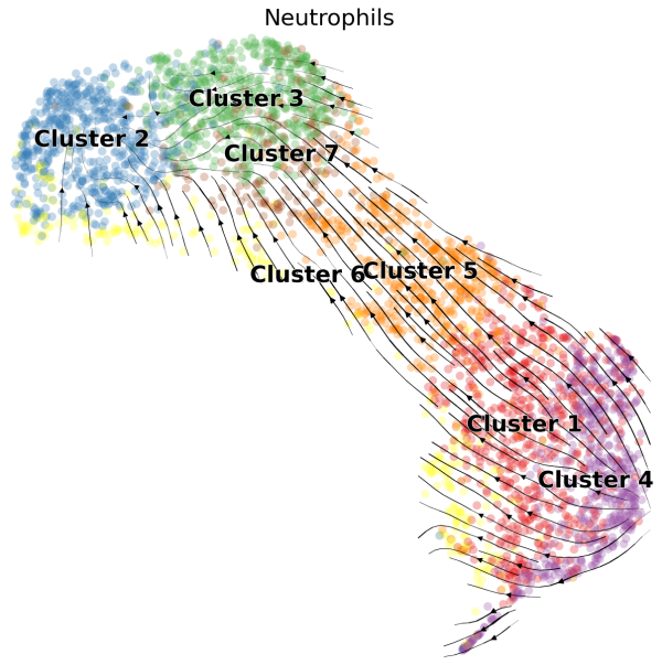
RNA velocity이란? 스플라이싱된 RNA와 아직 스플라이싱되지 않은 RNA를 구분해 세포의 상태를 예측하는 기법으로 scRNA 데이터에서 클러스터간에 분화 과정에 대한 단서를 얻을 수 있습니다. 예를 들어 아래 그림에서 보면 cluster4에서 cluster2로의 방향성을 확인 할 수 있습니다.

RNA velocity 분석을 위해서는 추가적으로 velocyto이라는 도구를 사용해 loom파일을 얻어야 합니다. 아래 명령어를 사용하면 간단하게 얻을 수 있습니다.

velocyto run10x run_count_mNeuron1k/ data/refdata-gex-mm10-2020-A/genes/genes.gtf

2023-09-19 10:01:22,756 - DEBUG - Using logic: Default
2023-09-19 10:01:22,757 - DEBUG - Example of barcode: AAACGAATCAAAGCCT and cell_id: run_count_mNeuron1k:AAACGAATCAAAGCCT-1
(중략)
2023-09-19 10:27:23,985 - DEBUG - 1991314 reads were skipped because no apropiate cell or umi barcode was found
2023-09-19 10:27:23,985 - DEBUG - Counting done!
2023-09-19 10:27:23,988 - DEBUG - Collecting row attributes
2023-09-19 10:27:24,014 - DEBUG - Generating data table
2023-09-19 10:27:24,056 - DEBUG - Writing loom file
2023-09-19 10:27:25,286 - DEBUG - Terminated Succesfully!

완료가 되면 run_count_mNeuron1k폴더안에 velocyto라는 새로운 폴더가 생기고 run_count_mNeuron1k.loom 파일이 생성됩니다.

6 Count matrix 데이터 읽기

6.1 Scanpy 사용

# conda install pandas scanpy
import scanpy as sc

# Cell ranger 결과 파일이 들어있는 경로
file_path = "../input/run_count_mNeuron1k/outs/filtered_feature_bc_matrix"

# read_10x_mtx 함수를 사용
adata = sc.read_10x_mtx(file_path, var_names="gene_symbols", cache=True)
adata

# conda install -c bioconda scvelo
import scvelo as scv

# load loom files for spliced/unspliced matrices for each sample
loom = scv.read(f"{file_path}/run_count_mNeuron1k.loom", validate=False, cache=False)

# rename barcodes in order to merge:
barcodes = [bc.split(":")[1] for bc in loom.obs.index.tolist()]
barcodes = [bc[0 : len(bc) - 1] + "-1" for bc in barcodes]
loom.obs.index = barcodes

# make variable names unique
loom.var_names_make_unique()

# merge matrices into the original adata object
adata = scv.utils.merge(adata, loom)
adata

scv.pl.proportions(adata)

adata.write("../output/mNeuron1k.h5ad", compression="gzip")

6.2 Seurat 사용

R에 좀 더 익숙하시다면 Seurat을 사용하세요. 저는 파이썬 문법을 더 좋아하지만 솔직히 분석 도구의 완성도 측면에서는 Seurat이 더 나은 것 같습니다. 아래 코드는 jupyter notebook에서 R코드를 사용하기 위해 필요한 것으로 rStudio를 사용하신다면 %%R이 포함된 셀의 코드만 사용하시면 됩니다.

import logging

import rpy2.rinterface_lib.callbacks as rcb

# import rpy2.robjects as ro

rcb.logger.setLevel(logging.ERROR)
%load_ext rpy2.ipython

%%R
library(dplyr)
library(Seurat)

%%R
# Load dataset
file_path <- "../input/run_count_mNeuron1k/outs/filtered_feature_bc_matrix"
neuron_data <- Read10X(data_dir=file_path)
# Initialize the Seurat object.
obj <- CreateSeuratObject(counts = neuron_data)
obj

Seurat object를 파일로 저장하는 방법에도 여러가지가 있지만 R에서 많이 사용되는 *.rds를 사용하는 코드는 아래와 같습니다.

%%R
saveRDS(obj, file = "../output/mNeuron1k.rds")

7 마치며

이것으로 scRNA seq 데이터의 전처리 과정을 알아봤습니다. 여기 적힌 방법 외에도 더 효율적이고 나은 방법도 있고 앞으로도 더 생겨날 것입니다. 그러나 저도 배우는 입장에서 다른 분들에게 도움이 되고자 정리를 해봤습니다. 실제 실험을 통해 얻은 데이터를 분석하는데 도움이 되길 바랍니다.