import os
import warnings

import numpy as np

warnings.filterwarnings("ignore")
np.random.seed(42)AutoGluon을 사용한 AutoML
Python
AWS
AutoGluon
MachineLearning
AutoML
AWS AI가 개발한 AutoGluon은 머신러닝 작업을 자동화하여 애플리케이션에서 강력한 예측 성능을 쉽게 달성할 수 있도록 지원합니다. 단 몇 줄의 코드만으로 이미지, 텍스트, 시계열 및 테이블 형식 데이터에 대해 높은 정확도의 머신러닝 및 딥러닝 모델을 학습하고 배포할 수 있습니다.
- 빠른 프로토타이핑: 몇 줄의 코드로 원시 데이터에 대한 머신러닝 솔루션을 구축합니다.
- 최첨단 기술: 전문가 지식 없이도 자동으로 SOTA 모델을 활용합니다.
- 쉬운 배포: 클라우드 예측기 및 사전 빌드된 컨테이너를 사용하여 실험에서 프로덕션으로 전환합니다.
- 사용자 정의 가능: 사용자 정의 기능 처리, 모델 및 메트릭으로 확장 가능합니다.
1 설치
AutoGluon은 Python 3.9 - 3.12을 지원되며 Linux, MacOS 및 Windows에서 사용할 수 있습니다. 다음과 같이 uv를 사용해 AutoGluon을 설치할 수 있습니다:
uv add autogluonGPU 지원, Conda 설치 및 선택적 종속성을 포함한 자세한 지침은 아래를 참조하십시오.
- https://auto.gluon.ai/stable/install.html
- https://github.com/autogluon/autogluon
2 테이블 형식 데이터 예측
AutoGluon의 TabularPredictor를 사용하여 테이블 형식 데이터셋의 다른 열을 기반으로 대상 열의 값을 예측하는 방법을 알아봅니다. 먼저 AutoGluon이 설치되었는지 확인한 다음 AutoGluon의 TabularDataset과 TabularPredictor를 가져옵니다. 전자는 데이터를 로드하는 데 사용하고 후자는 모델을 학습하고 예측하는 데 사용합니다.
from autogluon.tabular import TabularDataset, TabularPredictor2.1 예제 데이터
이 튜토리얼에서는 Nature 7887호의 커버 스토리인 수학 정리에 대한 AI 기반 직관의 데이터셋을 사용합니다. 목표는 매듭의 속성을 기반으로 매듭의 시그니처를 예측하는 것입니다. 원본 데이터에서 10K개의 학습 예제와 5K개의 테스트 예제를 샘플링했습니다. 샘플링된 데이터셋을 사용하면 이 튜토리얼을 빠르게 실행할 수 있지만, 원한다면 AutoGluon은 전체 데이터셋도 처리할 수 있습니다.
이 데이터셋을 URL에서 직접 로드합니다. AutoGluon의 TabularDataset은 pandas DataFrame의 하위 클래스이므로 모든 DataFrame 메서드를 TabularDataset에서도 사용할 수 있습니다.
data_url = "https://raw.githubusercontent.com/mli/ag-docs/main/knot_theory/"
train_data = TabularDataset(f"{data_url}train.csv")
train_data.head()| Unnamed: 0 | chern_simons | cusp_volume | hyperbolic_adjoint_torsion_degree | hyperbolic_torsion_degree | injectivity_radius | longitudinal_translation | meridinal_translation_imag | meridinal_translation_real | short_geodesic_imag_part | short_geodesic_real_part | Symmetry_0 | Symmetry_D3 | Symmetry_D4 | Symmetry_D6 | Symmetry_D8 | Symmetry_Z/2 + Z/2 | volume | signature | |
|---|---|---|---|---|---|---|---|---|---|---|---|---|---|---|---|---|---|---|---|
| 0 | 70746 | 0.090530 | 12.226322 | 0 | 10 | 0.507756 | 10.685555 | 1.144192 | -0.519157 | -2.760601 | 1.015512 | 0.0 | 0.0 | 0.0 | 0.0 | 0.0 | 1.0 | 11.393225 | -2 |
| 1 | 240827 | 0.232453 | 13.800773 | 0 | 14 | 0.413645 | 10.453156 | 1.320249 | -0.158522 | -3.013258 | 0.827289 | 0.0 | 0.0 | 0.0 | 0.0 | 0.0 | 1.0 | 12.742782 | 0 |
| 2 | 155659 | -0.144099 | 14.761030 | 0 | 14 | 0.436928 | 13.405199 | 1.101142 | 0.768894 | 2.233106 | 0.873856 | 0.0 | 0.0 | 0.0 | 0.0 | 0.0 | 0.0 | 15.236505 | 2 |
| 3 | 239963 | -0.171668 | 13.738019 | 0 | 22 | 0.249481 | 27.819496 | 0.493827 | -1.188718 | -2.042771 | 0.498961 | 0.0 | 0.0 | 0.0 | 0.0 | 0.0 | 0.0 | 17.279890 | -8 |
| 4 | 90504 | 0.235188 | 15.896359 | 0 | 10 | 0.389329 | 15.330971 | 1.036879 | 0.722828 | -3.056138 | 0.778658 | 0.0 | 0.0 | 0.0 | 0.0 | 0.0 | 0.0 | 16.749298 | 4 |
우리의 목표는 18개의 고유한 정수를 가진 “signature” 열에 저장됩니다. pandas가 이 데이터 유형을 범주형으로 올바르게 인식하지 못했지만 AutoGluon이 이 문제를 해결할 것입니다.
label = "signature"
train_data[label].describe()
count 10000.000000
mean -0.022000
std 3.025166
min -12.000000
25% -2.000000
50% 0.000000
75% 2.000000
max 12.000000
Name: signature, dtype: float642.2 학습
이제 레이블 열 이름을 지정하여 TabularPredictor를 구성한 다음 TabularPredictor.fit()으로 데이터셋에 대해 학습합니다. 다른 매개변수를 지정할 필요가 없습니다. AutoGluon은 이것이 다중 클래스 분류 작업임을 인식하고, 자동 특성 공학을 수행하고, 여러 모델을 학습한 다음, 모델을 앙상블하여 최종 예측기를 생성합니다.
predictor = TabularPredictor(label=label, verbosity=0).fit(train_data)모델 학습은 CPU에 따라 몇 분 또는 그 이하가 소요됩니다. time_limit 인수를 지정하여 학습 속도를 높일 수 있습니다. 예를 들어, fit(..., time_limit=60)은 60초 후에 학습을 중지합니다. 일반적으로 시간 제한이 길수록 예측 성능이 향상되며, 시간 제한이 너무 낮으면 AutoGluon이 합리적인 모델 세트를 학습하고 앙상블하는 것을 방해합니다.
2.3 예측
학습 데이터셋에 대해 학습된 예측기가 있으면 예측 및 평가에 사용할 별도의 데이터 세트를 로드할 수 있습니다.
test_data = TabularDataset(f"{data_url}test.csv")

y_pred = predictor.predict(test_data.drop(columns=[label]))
y_pred.head()
0 -4
1 0
2 0
3 4
4 2
Name: signature, dtype: int642.4 평가
evaluate() 함수를 사용하여 테스트 데이터셋에서 예측기를 평가할 수 있습니다. 이 함수는 모델 학습에 사용되지 않은 데이터에 대해 예측기가 얼마나 잘 수행되는지 측정합니다.
predictor.evaluate(test_data, silent=True){'accuracy': 0.9482,
'balanced_accuracy': np.float64(0.7448082022363894),
'mcc': np.float64(0.936511530000817)}AutoGluon의 TabularPredictor는 또한 leaderboard() 함수를 제공하여 테스트 데이터에 대한 각 개별 학습 모델의 성능을 평가할 수 있습니다.
predictor.leaderboard(test_data)| model | score_test | score_val | eval_metric | pred_time_test | pred_time_val | fit_time | pred_time_test_marginal | pred_time_val_marginal | fit_time_marginal | stack_level | can_infer | fit_order | |
|---|---|---|---|---|---|---|---|---|---|---|---|---|---|
| 0 | WeightedEnsemble_L2 | 0.9482 | 0.964965 | accuracy | 0.498636 | 0.403077 | 8.703081 | 0.004810 | 0.000391 | 0.042636 | 2 | True | 14 |
| 1 | LightGBM | 0.9456 | 0.955956 | accuracy | 0.019126 | 0.003349 | 1.833650 | 0.019126 | 0.003349 | 1.833650 | 1 | True | 5 |
| 2 | XGBoost | 0.9448 | 0.956957 | accuracy | 0.095466 | 0.010777 | 3.124414 | 0.095466 | 0.010777 | 3.124414 | 1 | True | 11 |
| 3 | LightGBMLarge | 0.9444 | 0.949950 | accuracy | 0.077716 | 0.014079 | 5.836701 | 0.077716 | 0.014079 | 5.836701 | 1 | True | 13 |
| 4 | CatBoost | 0.9432 | 0.955956 | accuracy | 0.024575 | 0.002570 | 7.570538 | 0.024575 | 0.002570 | 7.570538 | 1 | True | 8 |
| 5 | RandomForestEntr | 0.9384 | 0.949950 | accuracy | 0.189795 | 0.174759 | 0.604675 | 0.189795 | 0.174759 | 0.604675 | 1 | True | 7 |
| 6 | NeuralNetFastAI | 0.9376 | 0.944945 | accuracy | 0.053981 | 0.005054 | 3.912081 | 0.053981 | 0.005054 | 3.912081 | 1 | True | 3 |
| 7 | ExtraTreesGini | 0.9360 | 0.946947 | accuracy | 0.154584 | 0.212095 | 1.019274 | 0.154584 | 0.212095 | 1.019274 | 1 | True | 9 |
| 8 | ExtraTreesEntr | 0.9358 | 0.942943 | accuracy | 0.165139 | 0.191926 | 0.821660 | 0.165139 | 0.191926 | 0.821660 | 1 | True | 10 |
| 9 | NeuralNetTorch | 0.9352 | 0.949950 | accuracy | 0.013011 | 0.003917 | 126.092729 | 0.013011 | 0.003917 | 126.092729 | 1 | True | 12 |
| 10 | RandomForestGini | 0.9352 | 0.944945 | accuracy | 0.061000 | 0.176905 | 0.607355 | 0.061000 | 0.176905 | 0.607355 | 1 | True | 6 |
| 11 | LightGBMXT | 0.9320 | 0.945946 | accuracy | 0.036335 | 0.005550 | 2.252661 | 0.036335 | 0.005550 | 2.252661 | 1 | True | 4 |
| 12 | KNeighborsDist | 0.2210 | 0.213213 | accuracy | 0.014668 | 0.014991 | 0.017095 | 0.014668 | 0.014991 | 0.017095 | 1 | True | 2 |
| 13 | KNeighborsUnif | 0.2180 | 0.223223 | accuracy | 0.015354 | 0.016935 | 0.019544 | 0.015354 | 0.016935 | 0.019544 | 1 | True | 1 |
3 멀티모달 데이터 예측
AutoGluon의 MultiModalPredictor는 이미지, 텍스트, 테이블 형식 데이터를 포함한 입력을 위해 최첨단 딥러닝 모델을 자동으로 구축할 수 있는 모델 동물원의 딥러닝 모델 동물원입니다. 데이터를 AutoGluon의 멀티모달 데이터프레임 형식으로 변환하면 MultiModalPredictor가 다른 기능을 기반으로 한 열의 값을 예측할 수 있습니다.
3.1 예제 데이터
이 튜토리얼에서는 PetFinder 데이터셋의 단순화 및 서브샘플링된 버전을 사용합니다. 목표는 입양 프로필을 기반으로 애완동물 입양률을 예측하는 것입니다. 이 단순화된 버전에서 입양 속도는 0(느림)과 1(빠름)의 두 가지 범주로 그룹화됩니다. 먼저 petfinder 데이터셋이 포함된 zip 파일을 다운로드하고 현재 작업 디렉토리에 압축을 풉니다.
from autogluon.core.utils.loaders import load_zip

download_dir = "./ag_multimodal_tutorial"
zip_file = "https://automl-mm-bench.s3.amazonaws.com/petfinder_for_tutorial.zip"

load_zip.unzip(zip_file, unzip_dir=download_dir)
다음으로, pandas를 사용하여 데이터셋의 CSV 파일을 DataFrames으로 읽어들입니다. 예측하려는 열은 “AdoptionSpeed”입니다.
import pandas as pd

dataset_path = f"{download_dir}/petfinder_for_tutorial"

train_data = pd.read_csv(f"{dataset_path}/train.csv", index_col=0)
test_data = pd.read_csv(f"{dataset_path}/test.csv", index_col=0)

label_col = "AdoptionSpeed"
image_col = "Images"

train_data[image_col] = train_data[image_col].apply(lambda ele: ele.split(";")[0])
test_data[image_col] = test_data[image_col].apply(lambda ele: ele.split(";")[0])


def path_expander(path, base_folder):
    path_l = path.split(";")
    return ";".join([os.path.abspath(os.path.join(base_folder, path)) for path in path_l])


train_data[image_col] = train_data[image_col].apply(
    lambda ele: path_expander(ele, base_folder=dataset_path)
)
test_data[image_col] = test_data[image_col].apply(
    lambda ele: path_expander(ele, base_folder=dataset_path)
)
PetFinder 데이터셋에는 이미지 디렉토리가 있으며, 데이터의 일부 레코드에는 여러 이미지가 연결되어 있습니다. AutoGluon의 멀티모달 데이터프레임 형식에서는 이미지 열에 단일 이미지 파일 경로인 문자열이 포함되어야 합니다. 이 예에서는 이미지 특성 열을 첫 번째 이미지로만 제한하고 현재 디렉토리 구조에 맞게 모든 것을 올바르게 설정하기 위해 약간의 경로 조작이 필요합니다.
각 동물의 입양 프로필에는 사진, 텍스트 설명, 나이, 품종, 이름, 색상 등과 같은 다양한 테이블 형식 특성이 포함됩니다. 예제 데이터 행의 사진과 설명을 살펴보겠습니다.
from IPython.display import Image, display

example_row = train_data.iloc[0]
example_image = example_row[image_col]

pil_img = Image(filename=example_image)
display(pil_img)

example_row["Description"]
"I rescued Yumi Hamasaki at a food stall far away in Kelantan. At that time i was on my way back to KL, she was suffer from stomach problem and looking very2 sick.. I send her to vet & get the treatment + vaccinated and right now she's very2 healthy.. About yumi : - love to sleep with ppl - she will keep on meowing if she's hugry - very2 active, always seeking for people to accompany her playing - well trained (poo+pee in her own potty) - easy to bathing - I only feed her with these brands : IAMS, Kittenbites, Pro-formance Reason why i need someone to adopt Yumi: I just married and need to move to a new house where no pets are allowed :( As Yumi is very2 special to me, i will only give her to ppl that i think could take care of her just like i did (especially on her foods things).."3.2 학습
이제 데이터가 적절한 형식이 되었으므로 학습 데이터에 대해 MultiModalPredictor를 학습시킬 수 있습니다. 여기서는 이 빠른 데모를 위해 짧은 학습 시간 예산을 설정합니다. 학습 시간이 길수록 예측 성능이 향상되지만 짧은 시간 안에 놀라울 정도로 좋은 성능을 얻을 수 있습니다.
from autogluon.multimodal import MultiModalPredictor

predictor = MultiModalPredictor(label=label_col, verbosity=0).fit(
    train_data=train_data, time_limit=120
)
INFO: Seed set to 0
INFO: Using 16bit Automatic Mixed Precision (AMP)
INFO: GPU available: True (cuda), used: True
INFO: TPU available: False, using: 0 TPU cores
INFO: HPU available: False, using: 0 HPUs
INFO: You are using a CUDA device ('NVIDIA GeForce RTX 4090') that has Tensor Cores. To properly utilize them, you should set `torch.set_float32_matmul_precision('medium' | 'high')` which will trade-off precision for performance. For more details, read https://pytorch.org/docs/stable/generated/torch.set_float32_matmul_precision.html#torch.set_float32_matmul_precision
INFO: LOCAL_RANK: 0 - CUDA_VISIBLE_DEVICES: [0]
INFO:
| Name | Type | Params | Mode
------------------------------------------------------------------
0 | model | MultimodalFusionMLP | 207 M | train
1 | validation_metric | BinaryAUROC | 0 | train
2 | loss_func | CrossEntropyLoss | 0 | train
------------------------------------------------------------------
207 M Trainable params
0 Non-trainable params
207 M Total params
828.307 Total estimated model params size (MB)
1171 Modules in train mode
0 Modules in eval modeEpoch 0: 50%|█████ | 30/60 [00:03<00:03, 8.10it/s] INFO: Epoch 0, global step 1: 'val_roc_auc' reached 0.56208 (best 0.56208), saving model to '/mnt/c4a1c56d-0589-48cd-9717-f6c33a86fa3b/Tools/learn_autogluon/AutogluonModels/ag-20250718_065554/epoch=0-step=1.ckpt' as top 3Epoch 0: 100%|██████████| 60/60 [00:12<00:00, 4.99it/s]INFO: Epoch 0, global step 4: 'val_roc_auc' reached 0.75111 (best 0.75111), saving model to '/mnt/c4a1c56d-0589-48cd-9717-f6c33a86fa3b/Tools/learn_autogluon/AutogluonModels/ag-20250718_065554/epoch=0-step=4.ckpt' as top 3Epoch 1: 50%|█████ | 30/60 [00:02<00:02, 11.48it/s]INFO: Epoch 1, global step 5: 'val_roc_auc' reached 0.76056 (best 0.76056), saving model to '/mnt/c4a1c56d-0589-48cd-9717-f6c33a86fa3b/Tools/learn_autogluon/AutogluonModels/ag-20250718_065554/epoch=1-step=5.ckpt' as top 3Epoch 1: 100%|██████████| 60/60 [00:11<00:00, 5.39it/s]INFO: Epoch 1, global step 8: 'val_roc_auc' reached 0.78417 (best 0.78417), saving model to '/mnt/c4a1c56d-0589-48cd-9717-f6c33a86fa3b/Tools/learn_autogluon/AutogluonModels/ag-20250718_065554/epoch=1-step=8.ckpt' as top 3Epoch 2: 50%|█████ | 30/60 [00:02<00:02, 11.62it/s]INFO: Epoch 2, global step 9: 'val_roc_auc' reached 0.78306 (best 0.78417), saving model to '/mnt/c4a1c56d-0589-48cd-9717-f6c33a86fa3b/Tools/learn_autogluon/AutogluonModels/ag-20250718_065554/epoch=2-step=9.ckpt' as top 3Epoch 2: 100%|██████████| 60/60 [00:11<00:00, 5.27it/s]INFO: Epoch 2, global step 12: 'val_roc_auc' reached 0.79056 (best 0.79056), saving model to '/mnt/c4a1c56d-0589-48cd-9717-f6c33a86fa3b/Tools/learn_autogluon/AutogluonModels/ag-20250718_065554/epoch=2-step=12.ckpt' as top 3Epoch 3: 50%|█████ | 30/60 [00:02<00:02, 11.77it/s]INFO: Epoch 3, global step 13: 'val_roc_auc' reached 0.78417 (best 0.79056), saving model to '/mnt/c4a1c56d-0589-48cd-9717-f6c33a86fa3b/Tools/learn_autogluon/AutogluonModels/ag-20250718_065554/epoch=3-step=13.ckpt' as top 3Epoch 3: 100%|██████████| 60/60 [00:11<00:00, 5.36it/s]INFO: Epoch 3, global step 16: 'val_roc_auc' reached 0.78806 (best 0.79056), saving model to '/mnt/c4a1c56d-0589-48cd-9717-f6c33a86fa3b/Tools/learn_autogluon/AutogluonModels/ag-20250718_065554/epoch=3-step=16.ckpt' as top 3Epoch 4: 50%|█████ | 30/60 [00:02<00:02, 11.22it/s]INFO: Epoch 4, global step 17: 'val_roc_auc' reached 0.79222 (best 0.79222), saving model to '/mnt/c4a1c56d-0589-48cd-9717-f6c33a86fa3b/Tools/learn_autogluon/AutogluonModels/ag-20250718_065554/epoch=4-step=17.ckpt' as top 3Epoch 4: 100%|██████████| 60/60 [00:11<00:00, 5.13it/s]INFO: Epoch 4, global step 20: 'val_roc_auc' reached 0.79111 (best 0.79222), saving model to '/mnt/c4a1c56d-0589-48cd-9717-f6c33a86fa3b/Tools/learn_autogluon/AutogluonModels/ag-20250718_065554/epoch=4-step=20.ckpt' as top 3Epoch 5: 50%|█████ | 30/60 [00:02<00:02, 11.55it/s]INFO: Epoch 5, global step 21: 'val_roc_auc' was not in top 3Epoch 5: 100%|██████████| 60/60 [00:08<00:00, 7.18it/s]INFO: Epoch 5, global step 24: 'val_roc_auc' reached 0.80014 (best 0.80014), saving model to '/mnt/c4a1c56d-0589-48cd-9717-f6c33a86fa3b/Tools/learn_autogluon/AutogluonModels/ag-20250718_065554/epoch=5-step=24.ckpt' as top 3Epoch 6: 50%|█████ | 30/60 [00:02<00:02, 11.40it/s]INFO: Epoch 6, global step 25: 'val_roc_auc' reached 0.79764 (best 0.80014), saving model to '/mnt/c4a1c56d-0589-48cd-9717-f6c33a86fa3b/Tools/learn_autogluon/AutogluonModels/ag-20250718_065554/epoch=6-step=25.ckpt' as top 3Epoch 6: 100%|██████████| 60/60 [00:11<00:00, 5.26it/s]INFO: Epoch 6, global step 28: 'val_roc_auc' was not in top 3Epoch 7: 50%|█████ | 30/60 [00:02<00:02, 11.35it/s]INFO: Epoch 7, global step 29: 'val_roc_auc' was not in top 3
INFO: Time limit reached. Elapsed time is 0:02:02. Signaling Trainer to stop.Epoch 7: 52%|█████▏ | 31/60 [00:06<00:05, 4.98it/s]INFO: 💡 Tip: For seamless cloud uploads and versioning, try installing [litmodels](https://pypi.org/project/litmodels/) to enable LitModelCheckpoint, which syncs automatically with the Lightning model registry.Predicting DataLoader 0: 100%|██████████| 4/4 [00:00<00:00, 8.12it/s]INFO: 💡 Tip: For seamless cloud uploads and versioning, try installing [litmodels](https://pypi.org/project/litmodels/) to enable LitModelCheckpoint, which syncs automatically with the Lightning model registry.Predicting DataLoader 0: 100%|██████████| 4/4 [00:00<00:00, 8.38it/s]INFO: 💡 Tip: For seamless cloud uploads and versioning, try installing [litmodels](https://pypi.org/project/litmodels/) to enable LitModelCheckpoint, which syncs automatically with the Lightning model registry.Predicting DataLoader 0: 100%|██████████| 4/4 [00:00<00:00, 8.34it/s]내부적으로 MultiModalPredictor는 문제 유형(분류 또는 회귀)을 자동으로 유추하고, 특성 양식을 감지하고, 멀티모달 모델 풀에서 모델을 선택하고, 선택된 모델을 학습합니다. 여러 백본이 사용되는 경우 MultiModalPredictor는 그 위에 후기 융합 모델(MLP 또는 트랜스포머)을 추가합니다.
3.3 예측
모델을 학습시킨 후, 이를 사용하여 보류된 테스트 데이터셋의 레이블을 예측합니다.
predictions = predictor.predict(test_data.drop(columns=label_col))
predictions[:5]
INFO: 💡 Tip: For seamless cloud uploads and versioning, try installing [litmodels](https://pypi.org/project/litmodels/) to enable LitModelCheckpoint, which syncs automatically with the Lightning model registry.Predicting DataLoader 0: 100%|██████████| 4/4 [00:00<00:00, 11.89it/s]8 0
70 1
82 1
28 0
63 1
Name: AdoptionSpeed, dtype: int64분류 작업의 경우 각 출력 클래스에 대한 예측 확률을 쉽게 얻을 수 있습니다.
probs = predictor.predict_proba(test_data.drop(columns=label_col))
probs[:5]
INFO: 💡 Tip: For seamless cloud uploads and versioning, try installing [litmodels](https://pypi.org/project/litmodels/) to enable LitModelCheckpoint, which syncs automatically with the Lightning model registry.Predicting DataLoader 0: 100%|██████████| 4/4 [00:00<00:00, 12.30it/s]| 0 | 1 | |
|---|---|---|
| 8 | 0.998383 | 0.001617 |
| 70 | 0.000966 | 0.999034 |
| 82 | 0.000547 | 0.999453 |
| 28 | 0.999870 | 0.000130 |
| 63 | 0.005271 | 0.994729 |
3.4 평가
마지막으로, 보류된 테스트 데이터셋에서 다른 성능 메트릭, 이 경우 roc_auc에 대해 예측기를 평가할 수 있습니다.
scores = predictor.evaluate(test_data, metrics=["roc_auc"])
scores
INFO: 💡 Tip: For seamless cloud uploads and versioning, try installing [litmodels](https://pypi.org/project/litmodels/) to enable LitModelCheckpoint, which syncs automatically with the Lightning model registry.Predicting DataLoader 0: 100%|██████████| 4/4 [00:00<00:00, 11.93it/s]{'roc_auc': np.float64(0.8976)}4 시계열 데이터 예측
간단한 fit() 호출을 통해 AutoGluon은 다음을 학습하고 조정할 수 있습니다.
- 간단한 예측 모델 (예: ARIMA, ETS, Theta),
- 강력한 딥러닝 모델 (예: DeepAR, Temporal Fusion Transformer),
- 트리 기반 모델 (예: LightGBM),
- 다른 모델의 예측을 결합하는 앙상블
이를 통해 단변량 시계열 데이터에 대한 다단계 확률적 예측을 생성합니다.
이 튜토리얼에서는 AutoGluon을 사용하여 M4 예측 대회 데이터셋에 대한 시간별 예측을 빠르게 생성하는 방법을 보여줍니다.
4.1 시계열 데이터를 TimeSeriesDataFrame으로 로드하기
먼저 필요한 모듈을 가져옵니다.
import pandas as pd
from autogluon.timeseries import TimeSeriesDataFrame, TimeSeriesPredictorautogluon.timeseries를 사용하려면 다음 두 클래스만 필요합니다:
TimeSeriesDataFrame은 여러 시계열로 구성된 데이터셋을 저장합니다.TimeSeriesPredictor는 최상의 예측 모델을 피팅, 튜닝 및 선택하고 새로운 예측을 생성하는 작업을 처리합니다.
M4 시간별 데이터셋의 하위 집합을 pandas.DataFrame으로 로드합니다.
df = pd.read_csv(
    "https://autogluon.s3.amazonaws.com/datasets/timeseries/m4_hourly_subset/train.csv"
)
df.head()| item_id | timestamp | target | |
|---|---|---|---|
| 0 | H1 | 1750-01-01 00:00:00 | 605.0 |
| 1 | H1 | 1750-01-01 01:00:00 | 586.0 |
| 2 | H1 | 1750-01-01 02:00:00 | 586.0 |
| 3 | H1 | 1750-01-01 03:00:00 | 559.0 |
| 4 | H1 | 1750-01-01 04:00:00 | 511.0 |
AutoGluon은 시계열 데이터를 long format으로 예상합니다. 데이터 프레임의 각 행에는 다음으로 표시되는 단일 시계열의 단일 관측(타임스텝)이 포함됩니다.
- 시계열의 고유 ID(
"item_id") (int 또는 str) - 관측의 타임스탬프(
"timestamp") (pandas.Timestamp또는 호환 형식) - 시계열의 숫자 값(
"target")
원본 데이터셋은 항상 고유 ID, 타임스탬프 및 대상 값에 대한 최소 세 개의 열이 있는 이 형식을 따라야 하지만 이러한 열의 이름은 임의로 지정할 수 있습니다. 그러나 AutoGluon에서 사용하는 TimeSeriesDataFrame을 구성할 때 열 이름을 제공하는 것이 중요합니다. 데이터가 예상 형식과 일치하지 않으면 AutoGluon에서 예외가 발생합니다.
train_data = TimeSeriesDataFrame.from_data_frame(
    df, id_column="item_id", timestamp_column="timestamp"
)
train_data.head()| target | ||
|---|---|---|
| item_id | timestamp | |
| H1 | 1750-01-01 00:00:00 | 605.0 |
| 1750-01-01 01:00:00 | 586.0 | |
| 1750-01-01 02:00:00 | 586.0 | |
| 1750-01-01 03:00:00 | 559.0 | |
| 1750-01-01 04:00:00 | 511.0 |
TimeSeriesDataFrame에 저장된 각 개별 시계열을 _item_이라고 합니다. 예를 들어, 항목은 수요 예측의 다른 제품에 해당하거나 금융 데이터셋의 다른 주식에 해당할 수 있습니다. 이 설정은 시계열의 _패널_이라고도 합니다. 이것은 다변량 예측과 동일하지 않습니다. AutoGluon은 다른 항목(시계열) 간의 상호 작용을 모델링하지 않고 각 시계열에 대해 개별적으로 예측을 생성합니다.
TimeSeriesDataFrame은 pandas.DataFrame에서 상속되므로 pandas.DataFrame의 모든 속성과 메서드를 TimeSeriesDataFrame에서 사용할 수 있습니다. 또한 다양한 데이터 형식에 대한 로더와 같은 다른 유틸리티 기능도 제공합니다.
4.2 TimeSeriesPredictor.fit으로 시계열 모델 학습
시계열의 미래 값을 예측하려면 TimeSeriesPredictor 객체를 만들어야 합니다. autogluon.timeseries의 모델은 시계열을 미래의 _여러 단계_로 예측합니다. 우리는 작업에 따라 이러한 단계의 수, 즉 예측 길이(_예측 기간_이라고도 함)를 선택합니다. 예를 들어 우리 데이터셋에는 시간별 _빈도_로 측정된 시계열이 포함되어 있으므로 prediction_length = 48로 설정하여 미래 48시간까지 예측하는 모델을 학습합니다.
AutoGluon에 학습된 모델을 ./autogluon-m4-hourly 폴더에 저장하도록 지시합니다. 또한 AutoGluon이 평균 절대 스케일 오차(MASE)에 따라 모델 순위를 매겨야 하며 예측하려는 데이터가 TimeSeriesDataFrame의 "target" 열에 저장되도록 지정합니다.
predictor = TimeSeriesPredictor(
    prediction_length=48,
    path="autogluon-m4-hourly",
    target="target",
    eval_metric="MASE",
    verbosity=0,
)

predictor.fit(train_data, presets="medium_quality", time_limit=600)
<autogluon.timeseries.predictor.TimeSeriesPredictor at 0x73aacd597390>여기서는 "medium_quality" 사전 설정을 사용하고 학습 시간을 10분(600초)으로 제한했습니다. 사전 설정은 AutoGluon이 학습할 모델에 대한 파라미터를 정의합니다. medium_quality 사전 설정의 경우 다음과 같습니다.
- 간단한 기준선(
Naive,SeasonalNaive) - 통계 모델(
ETS,Theta) - LightGBM 기반 트리 기반 모델(
RecursiveTabular,DirectTabular) - 딥러닝 모델
TemporalFusionTransformer - 그리고 이들을 결합한 가중 앙상블입니다.
TimeSeriesPredictor에 사용할 수 있는 다른 사전 설정은
"fast_training","high_quality"및"best_quality"등이 있습니다.
사전 설정들은 일반적으로 더 정확한 예측을 생성하지만 학습하는 데 시간이 더 오래 걸립니다.
AutoGluon은 fit() 을 통해 주어진 시간 제한 내에서 가능한 한 많은 모델을 학습합니다. 그런 다음 학습된 모델은 내부 검증 세트에서의 성능을 기반으로 순위가 매겨집니다. 기본적으로 이 검증 세트는 train_data의 각 시계열에서 마지막 prediction_length 타임스텝을 제외하여 구성됩니다.
4.3 TimeSeriesPredictor.predict로 예측 생성
이제 학습된 TimeSeriesPredictor를 사용하여 미래 시계열 값을 예측할 수 있습니다. 기본적으로 AutoGluon은 내부 검증 세트에서 가장 좋은 점수를 받은 모델을 사용하여 예측합니다. 예측에는 항상 train_data의 각 시계열 끝에서 시작하여 다음 prediction_length 타임스텝에 대한 예측이 포함됩니다.
predictions = predictor.predict(train_data)
predictions.head()| mean | 0.1 | 0.2 | 0.3 | 0.4 | 0.5 | 0.6 | 0.7 | 0.8 | 0.9 | ||
|---|---|---|---|---|---|---|---|---|---|---|---|
| item_id | timestamp | ||||||||||
| H1 | 1750-01-30 04:00:00 | 622.354942 | 598.425139 | 606.981886 | 613.221995 | 617.991382 | 622.354942 | 627.043820 | 631.702888 | 637.264877 | 645.002394 |
| 1750-01-30 05:00:00 | 563.318481 | 537.515631 | 547.162459 | 553.498017 | 558.639161 | 563.318481 | 567.705346 | 572.642124 | 578.556409 | 587.001385 | |
| 1750-01-30 06:00:00 | 521.525187 | 494.325763 | 504.013476 | 511.095175 | 516.550982 | 521.525187 | 526.583225 | 532.032613 | 538.334244 | 547.525425 | |
| 1750-01-30 07:00:00 | 490.088652 | 461.432323 | 471.588108 | 478.747585 | 484.678311 | 490.088652 | 495.704356 | 501.733837 | 508.553248 | 519.106916 | |
| 1750-01-30 08:00:00 | 465.376269 | 435.200758 | 445.454704 | 452.924012 | 459.572474 | 465.376269 | 470.925032 | 477.133554 | 484.607983 | 495.218336 |
AutoGluon은 확률적 예측을 생성합니다. 미래의 시계열의 평균(기대값)을 예측하는 것 외에도 모델은 예측 분포의 분위수를 제공합니다. 분위수 예측은 가능한 결과의 범위에 대한 아이디어를 제공합니다. 예를 들어, "0.1" 분위수가 500.0과 같으면 모델은 대상 값이 500.0 미만일 확률이 10%라고 예측합니다.
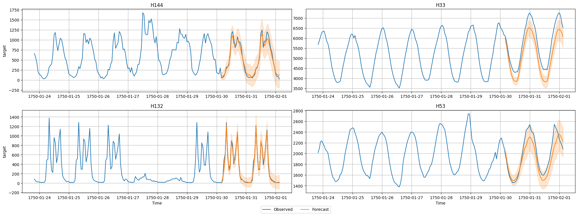
이제 데이터셋의 시계열 중 하나에 대한 예측과 실제 관측값을 시각화합니다. 잠재적 결과의 범위를 표시하기 위해 평균 예측과 10% 및 90% 분위수를 플로팅합니다.
test_data = TimeSeriesDataFrame.from_path(
    "https://autogluon.s3.amazonaws.com/datasets/timeseries/m4_hourly_subset/test.csv"
)

predictor.plot(
    test_data, predictions, quantile_levels=[0.1, 0.9], max_history_length=200, max_num_item_ids=4
);
4.4 다양한 모델의 성능 평가
leaderboard() 메서드를 통해 AutoGluon이 학습한 각 모델의 성능을 볼 수 있습니다. 테스트 데이터 세트를 리더보드 함수에 제공하여 학습된 모델이 보이지 않는 테스트 데이터에서 얼마나 잘 수행되는지 확인합니다. 리더보드에는 내부 검증 데이터셋에서 계산된 검증 점수도 포함됩니다.
테스트 데이터에는 예측 기간(각 시계열의 마지막 prediction_length 값)과 과거 데이터(마지막 prediction_last 값을 제외한 모든 값)가 모두 포함됩니다.
AutoGluon 리더보드에서 점수가 높을수록 항상 더 나은 예측 성능에 해당합니다. 따라서 MASE 점수에 -1을 곱하여 “음수 MASE”가 높을수록 더 정확한 예측에 해당하도록 합니다.
predictor.leaderboard(test_data)| model | score_test | score_val | pred_time_test | pred_time_val | fit_time_marginal | fit_order | |
|---|---|---|---|---|---|---|---|
| 0 | WeightedEnsemble | -0.697607 | -0.791366 | 13.339781 | 8.644861 | 0.386227 | 9 |
| 1 | Chronos[bolt_small] | -0.725739 | -0.812070 | 1.574927 | 1.777771 | 0.084811 | 7 |
| 2 | RecursiveTabular | -0.862797 | -0.933874 | 0.488657 | 0.336368 | 3.245855 | 3 |
| 3 | SeasonalNaive | -1.022854 | -1.216909 | 0.133975 | 0.105367 | 0.061909 | 2 |
| 4 | DirectTabular | -1.605700 | -1.292127 | 0.160719 | 0.166876 | 3.339360 | 4 |
| 5 | ETS | -1.806136 | -1.966098 | 10.985835 | 6.286225 | 0.059151 | 5 |
| 6 | Theta | -1.905367 | -2.142551 | 0.287385 | 0.309614 | 0.060678 | 6 |
| 7 | TemporalFusionTransformer | -2.065762 | -2.403856 | 0.125047 | 0.077620 | 33.022607 | 8 |
| 8 | Naive | -6.696079 | -6.662942 | 0.119962 | 1.052629 | 0.064250 | 1 |
4.5 요약
autogluon.timeseries를 사용하여 M4 시간별 데이터셋에 대한 확률적 다단계 예측을 수행했습니다. 시계열 예측을 위한 AutoGluon의 고급 기능에 대해 알아보려면 시계열 예측 - 심층 분석을 확인하십시오.
5 마치며
이 튜토리얼에서는 AutoGluon의 기능의 일부만 다루었습니다. AutoGluon은 테이블, 멀티모달, 시계열 등 다양한 데이터 유형에 대해 손쉽게 AutoML을 적용할 수 있는 강력한 오픈소스 프레임워크입니다. 이 튜토리얼에서는 TabularPredictor, MultiModalPredictor, TimeSeriesPredictor의 기본 사용법을 예제를 통해 데이터 준비, 모델 학습, 예측, 평가까지의 워크플로우로 살펴보았습니다.
AutoGluon을 활용하면 머신러닝 모델 개발의 진입 장벽을 크게 낮출 수 있으며, 실험에서 프로덕션까지의 전환도 매우 간편합니다. 더 깊이 있는 활용법과 고급 기능은 공식 문서와 심화 튜토리얼을 참고해보시기 바랍니다.